Abstract: Plane sweep is widely used in computational geometry, computer graphics, grid computing, and related areas. Many classic algorithms use plane sweep to greatly reduce time complexity — e.g. segment intersection, union of axis-aligned rectangle perimeters, rectangle intersection, spatial collision detection, Voronoi diagram construction, closest pair of points, and more.
This article introduces several plane sweep algorithms commonly used in ACM programming contests. By purpose, they fall into:
- Data aggregation;
- Detecting geometric positional relationships;
- Closest pair of points. We present representative classic algorithms from each category and analyze classic ACM contest problems, hoping to inspire contestants.
Keywords
Plane sweep ; ACM International Collegiate Programming Contest ; Algorithms ; Data aggregation ; Geometric positional relationships; Closest pair of points
Chapter 1: Introduction
The ACM International Collegiate Programming Contest (ACM-ICPC or ICPC), hosted by the Association for Computing Machinery (ACM), is an annual competition showcasing university students’ innovation, teamwork, and ability to program, analyze, and solve problems under pressure. After more than 30 years, ICPC has become one of the most influential university computer science contests.
The contest dates to 1970 at Texas A&M University, organized by the Alpha Chapter of the UPE Computer Science Honor Society. Universities across the US and Canada quickly adopted it as a way to discover top CS talent. In 1977 the first world finals were held during the ACM computer science conference; the event is now an annual international multi-country competition, with 35 editions held to date.
Plane sweep is an algorithmic optimization idea common in computational geometry and computer graphics. ACM contests demand very tight time and space bounds. Many geometry and advanced data structure problems can be optimized with plane sweep so solutions fit within limits.
A plane sweep algorithm typically has three parts: the sweep line, event points, and the active set on the current sweep line. The sweep line is usually horizontal (or vertical) and parallel to an axis. It processes event points top to bottom (or left to right), maintaining the active set by inserting or removing events. The active set is usually maintained with a segment tree, Fenwick tree, red-black tree, or other balanced BST; sometimes hash tables, sqrt decomposition, or skip lists are needed. Querying the active set yields the answer.
The body groups ACM sweep-line algorithms into three categories and introduces them in turn, hoping to help contestants learn these techniques.
Chapter 2: Algorithm Introduction and Problem Analysis
Section 1: Data Aggregation
Classic Problem A On the plane there are N axis-aligned rectangles (edges parallel to X or Y). Rectangles may partially or fully overlap. The perimeter of the union boundary is called the contour perimeter. E.g. in Figure 1 the contour of all rectangles is shown in Figure 2:
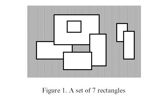
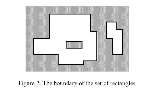
Design an algorithm to compute the contour perimeter of all rectangles.
Input N rectangles; rectangle i is given by lower-left (Xi, Yi) and upper-right (UXi, UYi).
Output Contour perimeter of all rectangles.
Algorithm analysis Discretize first. Cut the plane with the four lines of each rectangle. Then only unit segments like AB matter. Sum their lengths for total perimeter. Suppose vertical lines L1, L2 …, L8 map to mapx1, mapx2 …, mapx8. For convenience, let mapx0 = mapx1.
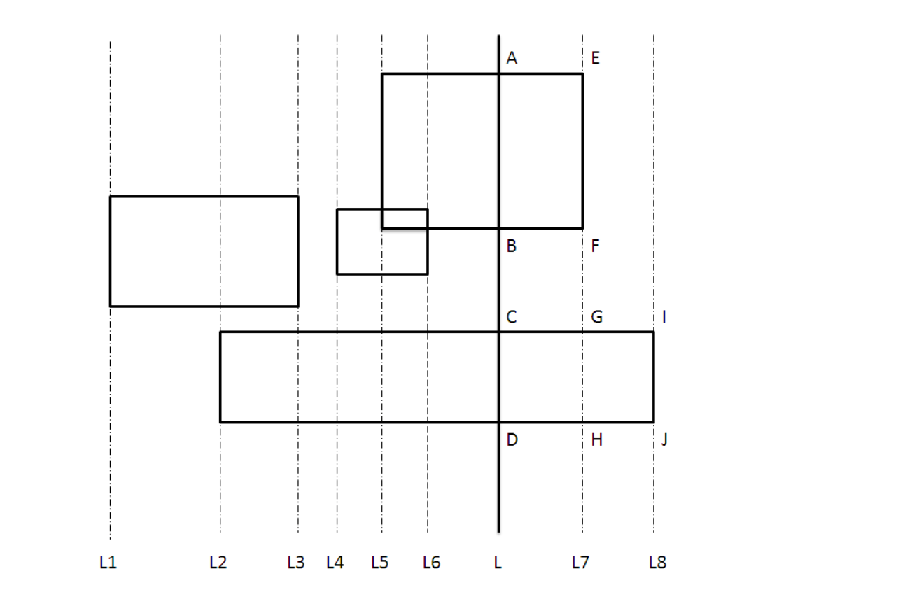
Consider horizontal unit segments between mapx(i-1) and mapxi that belong to the contour. Draw any vertical line L in [mapx(i-1), mapx(i)]; for all rectangles intersecting L, project onto L, take the union, and let count be the number of disjoint segments. Then horizontal contour length in that strip is 2count(mapxi - mapx(i-1)).
E.g. between L6 and L7, draw L; two rectangles project to AB and CD; union gives count=2, so horizontal contour length = 2count(L7-L6) = 4*(L7-L6).
The analysis above gives total horizontal contour length. Similarly for vertical length — but while sweeping vertical lines left to right, vertical contour length can be obtained more simply.
If projections on L7 are [E,F]∪[G,H] and on L8 are [I,J], when the sweep moves from L7 to L8, [E,F] “appears” as part of the vertical contour — exactly |projection on L7 − projection on L8|. If adjacent sweeps have projections M1, M2, exposed vertical edge length is |M1−M2|.
Summing horizontal and vertical contour lengths gives total perimeter.
Describe this with a sweep line moving left to right and updating state. The sweep line passes through vertical edges of rectangles. Event points are vertical edges: left edge = insert, right edge = delete. Inserts and deletes suggest maintaining the active set with a segment tree. SegmentTree should support:
//Initialize segment tree stree
1. void  Initialization(SegmentTree  stree);

//Insert segment [left,right] into stree
2. void  Insert(SegmentTree  stree , int  left , int  right) ;

//Delete interval [left,right] from stree (must have been inserted)
3. void  Delete(SegmentTree stree, int  left, int  right);

//Query count of disjoint segments after union of all active intervals
4. int  QueryCount(SegmentTree stree);

//Query total length after union of all active intervals
5. int  QueryTotalLength(SegmentTree stree);
Sweep algorithm for rectangle perimeter union [see Appendix A] (for how the segment tree implements these five operations, see reference [1]; omitted here):
0.  void rectangular_perimeter()
1.   Discretize coordinates from rectangle vertices; build mapx[0..2*N], mapy[0..2*N];
2.   Sort all events by x left to right.
3.   Initialization( stree ) ; //initialize segment tree
4.   nowTotalLength = 0 ;
5.   nowCount = 0 ;
6.   Answer = 0 ;
7.   for(i = 1 ; i <= 2*N ; ++ i){
8.         if( Event[i] is insert )
9.             Insert(stree , Event[i].down , Event[i].up ) ;//insert vertical segment [down,up]
10.        else
11.            Delete(stree , Event[i].down , Event[i].up ) ;//delete vertical segment [down,up]
12.        nowTotalLength = QueryTotalLength( stree ) ;
13.        nowCount = QueryCount( stree ) ;
14.        Answer = Answer + lastCount * 2 * (mapx[i] - mapx[i-1]) ;
15.        Answer = Answer + abs( nowTotalLength - lastTotalLength ) ;
16.        lastTotalLength = nowTotalLength ;
17.        lastCount = nowCount ;
18.  }
20.  return Answer ;
Complexity analysis With N rectangles, sorting in step 2 is O(NlogN). The segment tree supports insert, delete, query union length, and query disjoint segment count — each O(logN). N events total → O(NlogN).
Rectangle perimeter union is a classic plane sweep example. Many ACM problems extend it: sweep left to right, update state, read off the answer. Typical applications below.
Example A.1
N axis-aligned rectangles on the plane; find the area of their union. (POJ1151)
Algorithm analysis
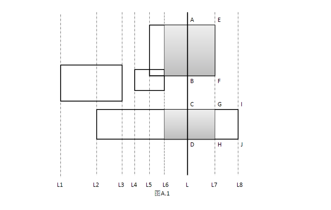
Previous problem: perimeter union; this one: area union. Very similar. Discretize as before; left vertical edge = insert, right = delete. As in Figure A.1, at sweep line L, project intersecting rectangles onto L as [A,B]∪[C,D]. Let length be the sum of projection lengths; area between L6 and L7 is length * (L7-L6). QueryTotalLength(stree) from the perimeter problem gives length directly. This problem is essentially a subproblem of the previous one — small changes suffice. [Code: Appendix A.1]
Complexity analysis
Same as above: O(NlogN).
Example A.2 You plan to grow vegetables on a large farm but hire n workers to plant seeds. Each worker plants one seed type on a rectangular plot. Plots may overlap, so overlapping regions get multiple seed types. Seeds compete; only the most competitive survives. More competitive seeds tend to yield higher-priced vegetables. Compute total revenue from selling all vegetables. (HDU 3255)
Input n(1<=n<=30000), m(1<=m<=3). n = workers, m = seed types. One line of m prices Price(i) for vegetable i (yuan per unit area). Then n lines with X1,Y1,X2,Y2,s: rectangle (X1,Y1)-(X2,Y2), seed type s.
Output Total revenue.
Algorithm analysis For worker i planting seed s on (X1,Y1,X2,Y2), imagine a box with base on the XOY plane and height Price(s). The problem becomes volume union of N such boxes. Slice with planes z=Price(i); area Area(i) of the cross-section is rectangle area union (Example A.1).
Total volume = sigma{Area(i) * [Price(i) - Price(i-1)]}, Price(0)=0.
Complexity analysis Worst case each slice hits N rectangles; area union O(NlogN) per slice, m slices → O(MNlogN). [Code: Appendix A.2]
Example A.3 (HDU 3621) N axis-aligned rectangles; find area covered by exactly K rectangles.
Input First line N(1<=N<=10000), K(1<=K<=N); Then N lines X1,Y1,X2,Y2 per rectangle.
Output Area covered by exactly K rectangles.
Algorithm analysis Looks like Example A.1 with K=1 generalized to arbitrary K.
Sweep line and events are the same. But Example A.1 relies on fast insert/delete/query union length on a segment tree; a segment tree cannot quickly query length covered by exactly K segments. Need another structure supporting: insert segment, delete segment, query length covered by exactly K segments.
Sqrt decomposition (block list) works well. Split the Y axis into blocks of length ~sqrt(N). A segment’s middle covers whole blocks; ends are handled element-wise. Per block, hash H stores length covered i times as H(i), and q = whole-block coverage count. Query H(k-q) per block.
Complexity analysis Each of the three operations costs O(sqrt(N)) → total O(N*sqrt(N)). [Code: Appendix A.3]
Classic Problem B N points (x,y) each with weight. A rectangle of height H, width W, axis-aligned — where to place it to maximize the sum of weights of covered points (points on the boundary count as outside)?
Input First line: N, W, H. Then N lines (x,y,weight).
Output Maximum weight sum inside the rectangle.
Algorithm analysis Two sweep lines Left, Right scan points while keeping horizontal distance ≤ W−1. See Figure B1.
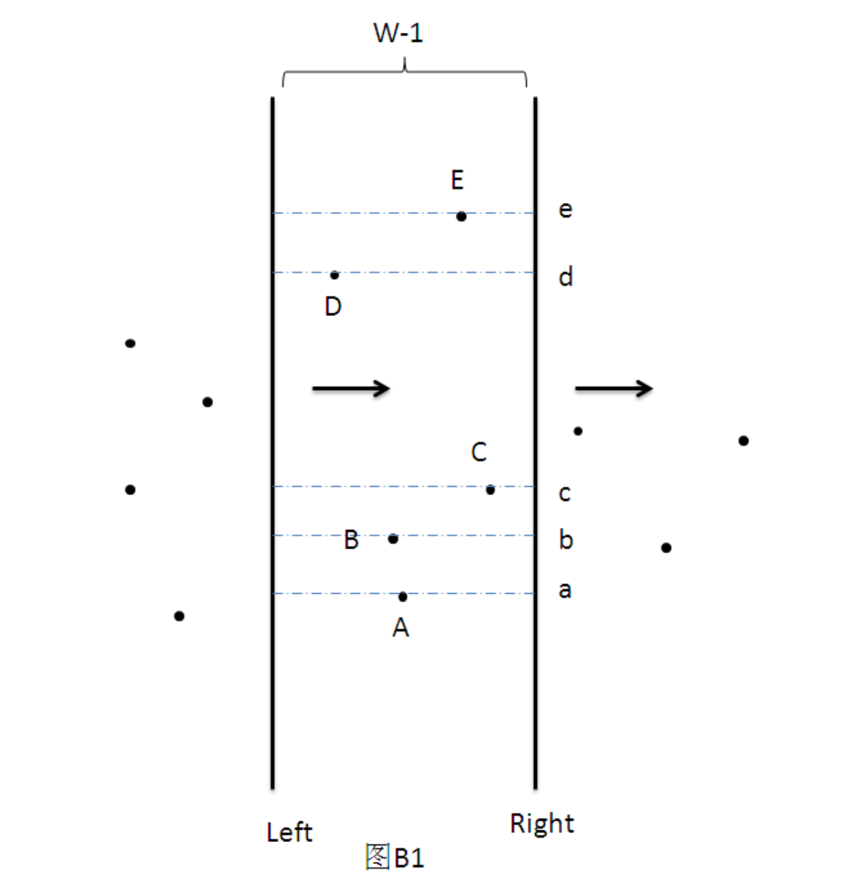
For points with x in [Left, Right], e.g. S={A,B,C,D,E} in Figure B1, map to the Y axis: MAPy(S)={a,b,c,d,e}.
Problem becomes: on a 1D axis with K points and a segment of length H, where to place the segment to maximize covered weight sum?
In Figure B2, S={a,b,c,d,e}, weights W={3,2,5,6,3}. Split each point x into x and x+H with weights w(x) and −w(x): S1={a,a+H,b,b+H,c,c+H,d,d+H,e,e+H}, W1={3,-3,2,-2,5,-5,6,-6,3,-3}
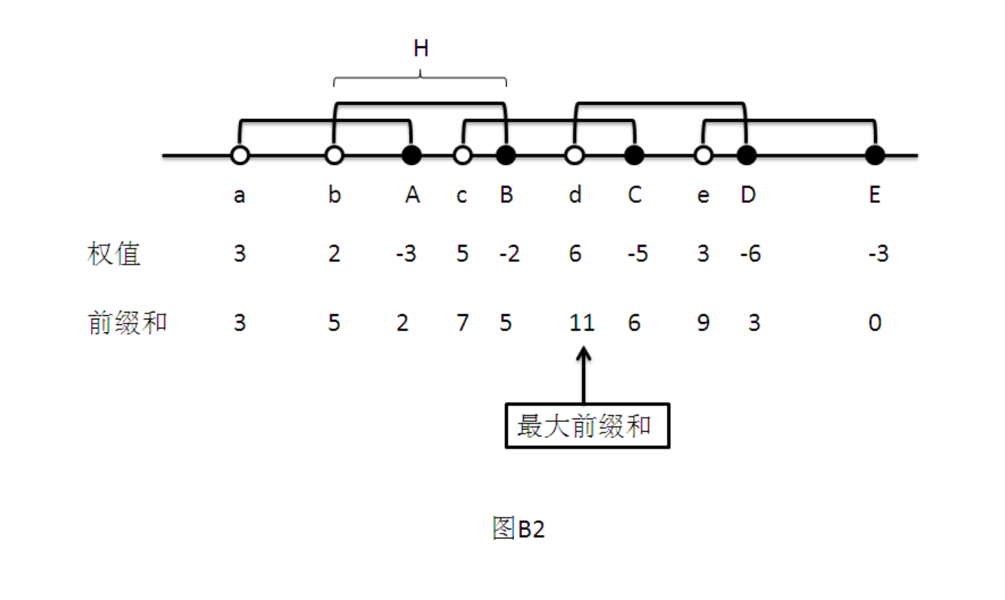
Sort by position; maximum prefix sum is the answer. +w(x) = point enters the length-H window; −w(x) = point leaves. Moving the window left to right equals computing prefix sums.
Algorithm: two vertical sweeps Left, Right; maintain points between them with a segment tree or balanced BST; query max prefix sum.
Tree must support:
void  Init(); //initialize;
void  Insert(int  x ,int  weight_x); //insert point x with weight weight_x ;
void  Delete(int  x,int  weight_x);//delete point x with weight weight_x ;
int  Max_Prefix() ;//max prefix sum of current sequence;
Init: O(n); insert/delete: O(logn); Max_Prefix: O(1).
0.     int Max_Cover(Point p[] , int n , int W , int H)
1.        Discretize {p[0].y , p[0].y+H , ... , p[n-1].y , p[n-1].y + H } to my[] ;
2.        Sort p[0..n-1] by x;
3.        tree.init() ;
4.        cur = ans = 0 ;
5.        for(i = 0 ; i < n ; ++ i){
6.            for(; cur < n ; ++ cur)
7.              if(p[cur].x - p[i].x < W ){
8.                    tree.Insert(  my[ p[cur].y ]   , p[cur].w ) ;
9.                    tree.Delete(  my[ p[cur].y+H ] , p[cur].w ) ;
10.                   ans = max(ans , tree.Max_Prefix() ) ;
11.             }else break ;
12.           tree.Insert(my[p[i].y]   ,  p[i].w );
13.           tree.Delete(my[p[i].y+H] ,  p[i].w ) ;
14.       }
15.       return ans ;
Complexity analysis Line 1: discretization O(NlogN). Line 2: sorting O(NlogN). Lines 6–11: cur only increases; each point enters tree once. Total: O(NlogN). [Code: Appendix B]
Section 2: Detecting Geometric Positional Relationships
Classic Problem C N axis-aligned rectangles. Design an efficient algorithm to detect whether any two intersect (at least one common point; containment counts as intersection).
Algorithm analysis Same spirit as Example A.1: discretize with rectangle edges; vertical sweep line; left edge = insert, right = delete. On insert, check whether the new segment intersects any active segment; if yes, two rectangles intersect. Otherwise insert. On delete, just delete.
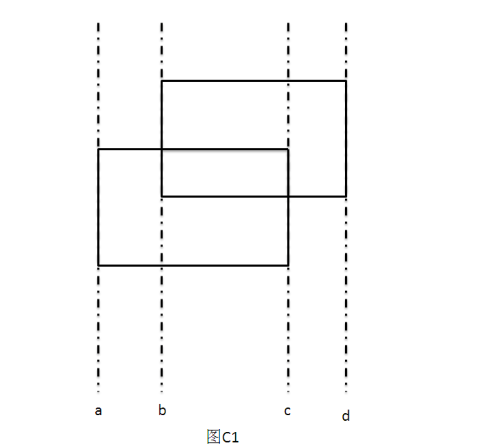
Use a segment tree for fast intersection tests. Operations (implementation details omitted):
//Initialize segment tree;
void  Init() ;

//Insert segment [left,right];
void  Insert(int  left , int  right);

//Delete segment [left,right];
void  Delete(int  left , int  right);

//Whether any active segment intersects [left,right]
void  hasIntersect(int  left , int  right);
Algorithm:
00.     boolean has_rectangle_intersect(rectangle r[] , int n)
01.         Discretize {r[0].left_x , r[0].right_x , ... ,
                  r[n-1].left_x , r[n-1].right_x} to mapx[] ;
02.         for( i = 0 ; i < n ; ++ i){
03.             event[i<<1]     = {r[i].left_x , r[i].down_y , r[i].up_y , +1 } ;
04.             event[(i<<1)|1] = {r[i].right_x, r[i].down_y , r[i].up_y , -1 } ;
05.         }
06.         Sort event[0..2*n-1] by x;
07.         tree.init() ; //initialize segment tree
08.         for( i = 0 ; i < n<<1 ; ++ i){
09.             if( event[i] is insert ){
10.                 if( tree.hasIntersection(event[i].down_y , event[i].up_y) )
11.                         return true ;
12.                 tree.Insert(event[i].down_y , event[i].up_y) ;
13.             }else{
14.                 tree.Delete(event[i].down_y , event[i].up_y);
15.             }
16.         }
17.         return false ;
Complexity analysis
Line 1: discretization O(NlogN). Line 6: event sort O(NlogN). Lines 8–16: O(logN) per event, 2N events → O(NlogN). Total: O(NlogN).
Classic Problem D N circles in the plane; any two are either nested or disjoint. Given centers and radii, find nesting relationships. Represent nesting as a tree: if A is inside B, draw A→B; B is parent of A. Figure D1 → D2 (R is an infinite circle containing all N).
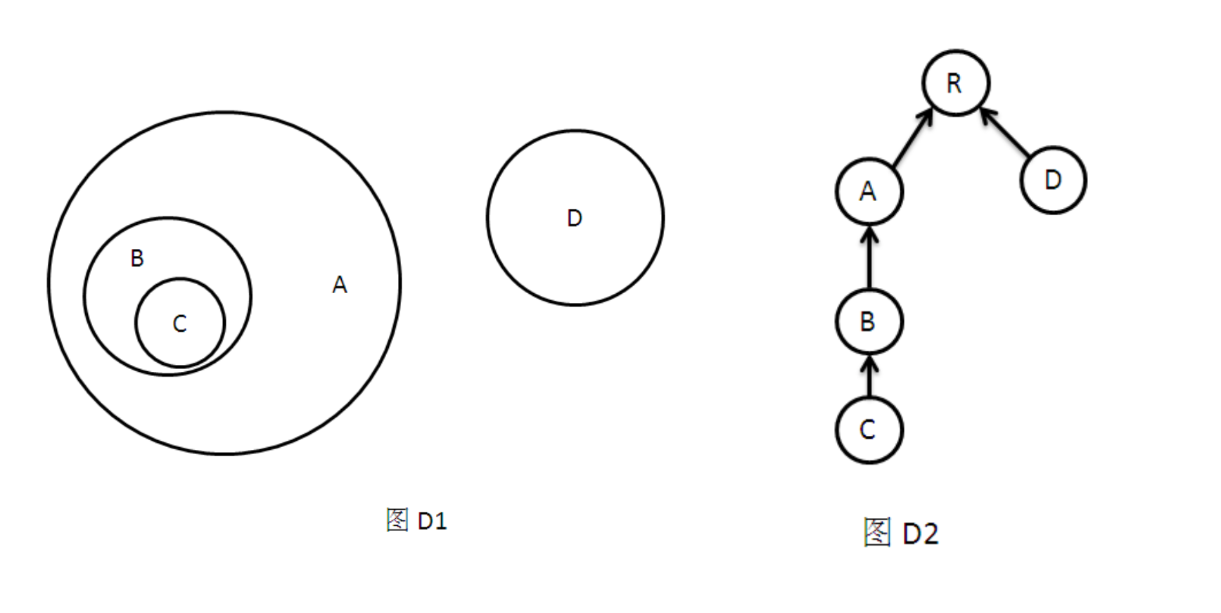
Algorithm analysis Imagine a vertical sweep line moving left to right. For circle (Xi,Yi,Ri), add events (Xi-Ri,Yi,-1) and (Xi+Ri,Yi,+1) for entering and leaving the sweep. At any time, each other circle has 0 or 2 intersections with the sweep (tangency = two coincident points). A balanced tree stores intersection y-positions, marked +1 (upper) or −1 (lower). Process events by increasing x. On enter (Xi-Ri,Yi,-1) for circle A, find minimum enclosing circle (parent): in the tree, largest intersection below Yi; if lower endpoint, that circle B is parent of A (Figure D3). If upper endpoint, B is sibling; parent of A is parent of B (Figure D4).
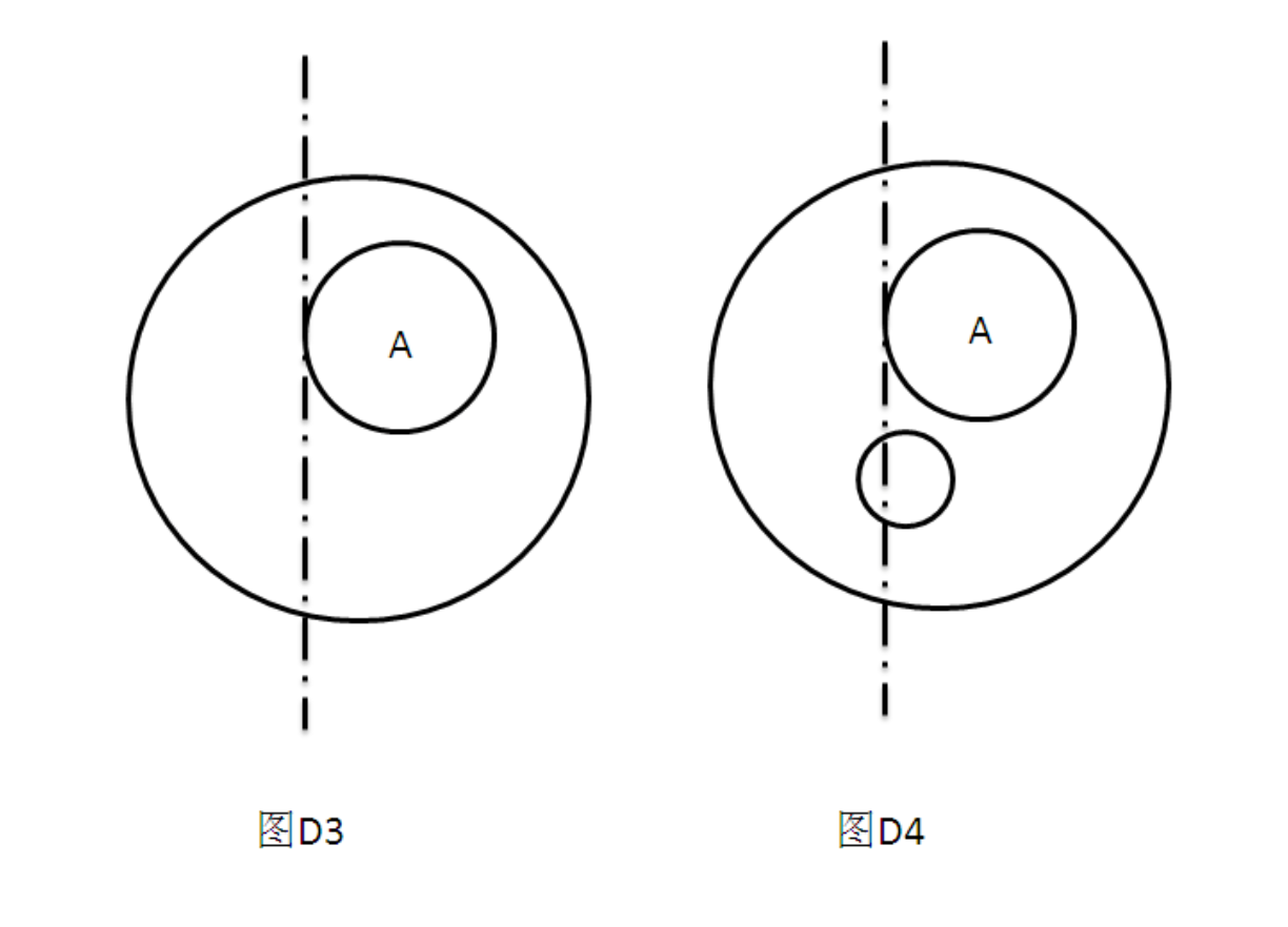
After finding parent, insert A’s two intersections. On leave event, delete them. After all events, tree structure is built (parent pointers).
00.  int[]  build_tree(circle c[] , int n)
01.           for(i = 0 ; i < n ; ++ i){
02.               event[2*i]   = {i , c[i].x - c[i].r , c[i].y , -1 } ;
03.               event[2*i+1] = {i , c[i].x - c[i].r , c[i].y , +1 } ;
04.           }
05.           Sort event[0..2*n-1] by x (insert before delete on tie);
06.           tree.init() ; //initialize tree structure
07.           for(i = 0 ; i < 2*n ; ++i){
08.                if(event[i] is delete){
09.                      tree.Delete( upper intersection of this event );
10.                      tree.Delete( lower intersection of this event );
11.                }
12.                if(event[i] is insert){
13.                      tree.Insert( upper intersection of this event );
14.                      tree.Insert( lower intersection of this event );
15.                      Down = tree.Below( lower intersection of this event ) ;
16.                      if( Down == NULL ){
17.                           father[ circle of current event ] = infinite circle;
18.                      }else{
19.                           if( Down is upper intersection )
20.                              father[ circle of current event ] = father[ circle of Down ] ;
21.                           if( Down is lower intersection )
22.                              father[ circle of current event ] = circle of Down;
23.                      }
24.                }
25.           }
26.           return father ;
Complexity analysis
Line 5: sort 2N events O(NlogN). Lines 7–25: insert/delete/query per event O(logN) → O(NlogN). Total: O(NlogN). [Code: Appendix D]
Section 3: Closest Pair of Points
Classic Problem E N points in the plane; compute closest-pair distance efficiently.
Algorithm analysis Closest pair is a classic divide-and-conquer problem in computational geometry; lower bound O(NlogN) is known. Reference [2] details divide-and-conquer. Compared to that, the sweep-line solution is more concise. Both rely on an important theorem:
Theorem Let p(1),…,p(n) be sorted by x. Let d(i) be closest-pair distance among p(1),…,p(i). Given d(i-1), to compute d(i) we need at most 6 points to the left of p(i) to possibly improve d(i).
Proof Clearly d(i) ≤ d(i-1). If adding p(i) yields a closer pair, p(i) must be closer than d(i-1) to some p(j) among p(1),…,p(i-1). Such points lie only in S = [p(i).x-d(i-1), p(i).x] × [p(i).y-d(i-1), p(i).y+d(i-1)]. We show S cannot contain more than 6 points.
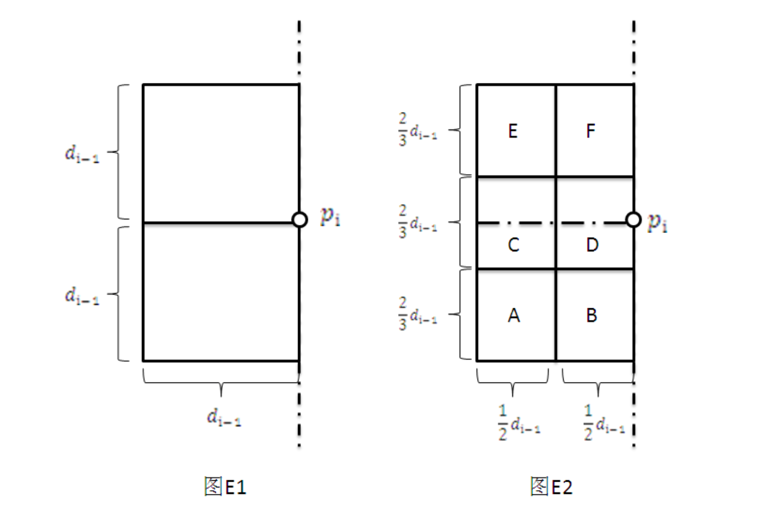
Proof by contradiction. If more than 6 points in S, partition S into 6 subregions as shown, each of size:
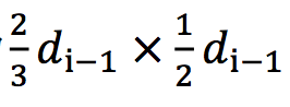
By pigeonhole, two points p(j), p(k) lie in the same subregion. Then
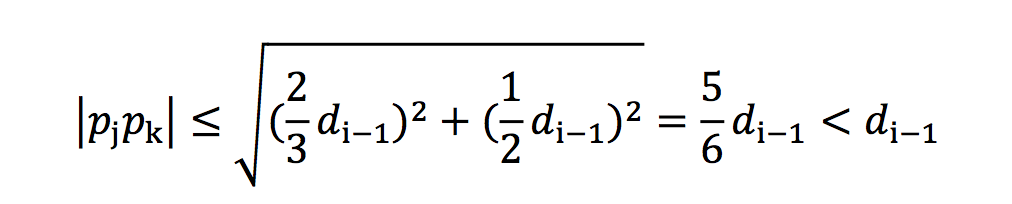
So among p(1),…,p(i-1) we found p(j), p(k) closer than d(i-1), contradicting the definition of d(i-1).
Theorem proved.
By the theorem, when updating d(i), compare p(i) to at most 6 neighbors. How to find those “left neighbors”? Sweep vertically left to right; maintain neighbors in a balanced BST ordered by y (smaller y first). BST supports:
Init();//initialize BST
Insert(Point p); //insert point p
Delete(Point p); //delete point p
Lower_Bound(Point p);//smallest point in BST not less than p
0.     double closest_point(Point p[] , int n)
1.     Sort p[1]..p[n] by x;
2.     BST.Init() ; // initialize BST
3.     BST.Insert( p[1] ) ; //insert first point
4.     left = 0 ;
5.     distance = infinity  ; //initialize closest distance
6.     for( i = 2 ; i <= n ; ++ i){
7.        //keep all BST points within horizontal distance distance of p[i]
8.         while(left <= n && p[i].x - p[left].x >= distance )
10.            BST.Delete( p[left] ) ;
11.         q = BST.Lower_Bound( Point(p[i].x ,p[i].y-distance )) ;
12.         while( q != BST.end()  && q.y - p[i].y < distance ) {
13.                 //compute and update distance .
14.                 distance = min(distance , dist( q , p[i])) ;
15.                 q = BST.next(q)  ; //successor of q
16.         }
17.    }
18.    return distance ;
Complexity analysis
Chapter 3: Conclusion
Plane sweep is a central algorithm design idea. By exploiting locality between objects, it clarifies problem structure and optimizes complexity.
This paper analyzes five classic problems across data aggregation, geometric relationship detection, and closest pair, with corresponding contest problems. Each has clear algorithm flow and complexity analysis, with proofs where needed.
Typical sweep algorithms have three parts: sweep line, events (usually insert/delete), and a structure for the active set (balanced BST, segment tree; sometimes block list or skip list). Sort events, sweep in order, maintain the active set per event type, query it for the answer. Answers emerge while processing adjacent events.
Sweep line has many more applications — spatial collision detection, Voronoi diagrams, computer graphics, as noted in the abstract.
References
[1] “Choosing Data Structures for Algorithm Efficiency — From IOI98 PICTURE” by Chen Hong [2] “Algorithm Design and Analysis” by Wang Xiaodong [3] “Solutions to ICPC Example Problems (VI)” by Guo Songshan, Weng Yujian, Liang Zhirong, Wu Yi [4] “The Art of Algorithms and Informatics Competitions” by Liu Rujia, Huang Liang [5] “Computational Geometry: Algorithm Design and Analysis” by Zhou Peide [6] “Computational Geometry: Algorithms and Applications” by Berg, M. et al., translated by Deng Junhui
Appendix
- Classic Problem A: Rectangle contour perimeter
- Example A.1: Union area of axis-aligned rectangles
- Example A.2: Farming from HDU 3255
- Example A.3: Area K from HDU 3621
- Classic Problem B: Max weight covered by a fixed rectangle
- Classic Problem D: Nesting of circles in the plane
- Classic Problem E: Closest pair in the plane